Induced Dipole#

Energy#

\(\mu\) is the induced dipole in the external field E. The induced field due to the induced dipole is \(E^u=-T\mu\), and the induced dipole is proportional to the total field \(E^t\):

\[\mu = \alpha E^t = \alpha(E+E^u),\]

where \(\alpha\) is the polarizability. Defining \(\tilde{T}=\alpha^{-1}+T\), the induced dipole is the solution to the linear equation

(5)#\[\tilde{T}\mu = E.\]

The polarization energy is given by

(6)#\[\begin{split}U &= -\mu E +\int_0^\mu d\mu\ \tilde{T}\mu \\ &= -\mu E +\frac{1}{2}\mu\tilde{T}\mu.\end{split}\]

On the right-hand side of (6):

the 1st term is the contribution from the external field;

the 2nd term is the mutual and self polarization energy.

Finally, the polarization energy is

(7)#\[U = -\frac{1}{2}\mu E.\]

Gradient#

With limited numerical precision, the solution to linear equation (5) cannot be fully precise:

(8)#\[\tilde{T}\mu = \epsilon + E.\]

The gradient of the induced dipole can be written in

\[\mu' = \tilde{T}^{-1}(\epsilon' + E' - \tilde{T}'\mu),\]

and the polarization gradient is

\[\begin{split}U' &= -\frac{1}{2} (E\mu' + \mu E') \\ &= -\frac{1}{2} [(-\epsilon+\mu\tilde{T})\tilde{T}^{-1}(\epsilon' +E' -\tilde{T}'\mu) +\mu E'] \\ &\approx -\frac{1}{2} (\mu E' -\mu\tilde{T}'\mu +\mu E'),\end{split}\]

only if the convergence of (8) is tight that \(\epsilon\) and \(\epsilon'\) terms will drop.

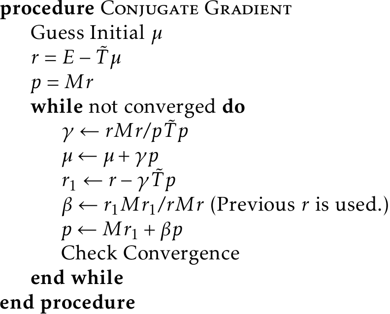
Conjugate Gradient#

Tinker uses the following Conjugate Gradient algorithm (C.G.) with a sparse matrix preconditioner (denoted as M) [7] to obtain the induced dipoles. Related Tinker variables and routines are tabulated.

C.G. Terms	Tinker variables and routines
\(\gamma\)	a
\(\beta\)	b
\(r\)	rsd
\(M r\)	zrsd
\(p\)	conj
\(\tilde{T} p\)	vec
\(-T\)	ufield()
\(M\)	uscale()

Polarization Model: AMOEBA (Thole Damping 2)#

AMOEBA force field adopts two polarization schemes, d and p, for the external field due to the permanent multipoles, and a third scheme u for mutual induced dipole interactions. Both d and u schemes are group-based. The p scheme is atomic connectivity-based. Tinker uses C.G. iterations to solve the following linear equations

\[\begin{split}(1/\alpha+T^u)\mu_d &= E_d \\ (1/\alpha+T^u)\mu_p &= E_p,\end{split}\]

and defines the polarization energy as

(9)#\[U = -\frac{1}{2}\mu_d E_p.\]

From an optimizational perspective, (9) is the minimum of the target function

\[f_1(\mu_d,\mu_p)=\frac{1}{2}\left(\frac{1}{2}\mu_d\tilde{T}\mu_p +\frac{1}{2}\mu_p\tilde{T}\mu_d -E_d\mu_p-E_p\mu_d\right),\]

whereas the way C.G. coded in Tinker is to solve the minimum of another target function

\[f_2(\mu_d,\mu_p)=\frac{1}{2}\left(\frac{1}{2}\mu_d\tilde{T}\mu_d +\frac{1}{2}\mu_p\tilde{T}\mu_p -E_d\mu_d-E_p\mu_p\right).\]

The difference in two target functions is usually negligible unless other loose convergence methods are used to compute the induced dipoles.

In the Thole damping model, a charge distribution \(\rho\) is used as a replacement for the point dipole model. AMOEBA adopts the second functional form

\[\rho = \frac{3a}{4\pi}\exp(-au^3)\]

from paper [8], where u is the polarizability-scaled distance. The electrostatic field and potential at distance r can be obtained from Gauss’s law,

\[E(r) = -\phi'(r) = \frac{1}{r^2} \int_0^u du\ 4\pi u^2 \rho = \frac{1-\exp(-au^3)}{r^2},\]

\[\phi(r) = \int_r^\infty dr\ E(r) = \frac{\lambda_1}{r} = \frac{1}{r}\left[ 1-\frac{(au^3)^\frac{1}{3}}{3}\Gamma(-\frac{1}{3},au^3)\right],\]

where \(\lambda_1\) serves as the \(B_0\) term in EWALD quadrupole interactions. \(\lambda_n\) terms are also related via derivatives

\[\begin{split}\phi'' &= \frac{1}{r^3}\left[2-(2+3au^3)\exp(-au^3)\right], \\ \phi''' &= \frac{3}{r^4}\left[-2+(2+2au^3+3a^2u^6)\exp(-au^3)\right], \\ \phi'''' &= \frac{3}{r^5}\left[8-(8+8au^3+9a^3u^9)\exp(-au^3)\right],\end{split}\]

\[\begin{split}\phi'_i &= \phi'\frac{r_i}{r}, \\ \phi''_{ij} &= \left(\phi''-\frac{\phi'}{r}\right)\frac{r_i r_j}{r^2} +\frac{\phi'}{r}\delta_{ij}, \\ \phi'''_{ijk} &= \left(\phi'''-\frac{3\phi''}{r}+\frac{3\phi'}{r^2}\right)\frac{r_i r_j r_k}{r^3} +\left(\frac{\phi''}{r}-\frac{\phi'}{r^2}\right)\frac{\sum r_k \delta_{ij}}{r}, \\ \phi''''_{ijkl}&= \left(\phi''''-\frac{6\phi'''}{r}+\frac{15\phi''}{r^2}-\frac{15\phi'}{r^3}\right) \frac{r_i r_j r_k r_l}{r^4} \\ &+\left(\frac{\phi'''}{r}-\frac{3\phi''}{r^2}+\frac{3\phi'}{r^3}\right)\frac{\sum r_k r_l\delta_{ij}}{r^2} +\left(\frac{\phi''}{r^2}-\frac{\phi'}{r^3}\right)\sum\delta_{kl}\delta_{ij}.\end{split}\]

Thus,

\[\begin{split}-\lambda_3/r^3 &= \phi'/r \Rightarrow \\ &\lambda_3 = 1 - \exp(-au^3), \\ 3\lambda_5/r^5 &= (\phi''-\phi'/r)/r^2 \Rightarrow \\ &\lambda_5 = 1 - (1+au^3)\exp(-au^3), \\ -15\lambda_7/r^7 &= (\phi'''-3\phi''/r+3\phi'/r^2)/r^3 \Rightarrow \\ &\lambda_7 = 1 - \left(1+au^3+\frac{3}{5}a^2 u^6\right)\exp(-au^3), \\ 105\lambda_9/r^9 &= (\phi''''-6\phi'''/r+15\phi''/r^2-15\phi'/r^3)/r^4 \Rightarrow \\ &\lambda_9 = 1 - \left(1+au^3+\frac{18}{35}a^2 u^6+\frac{9}{35}a^3 u^9\right)\exp(-au^3).\end{split}\]

Permanent Multipole

Quasi-Internal Frame